Fasttext for Knowledge Graph Embeddings
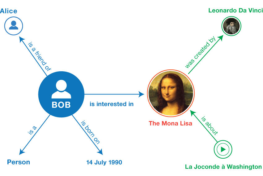
Knowledge Graphs are highly flexible data structures that are used to represent relationships between real world entities. Entities such as "Mona Lisa", or "DaVinci", are represented as nodes in the graph, while relationships such as "created_by", are represented as edges.
These graphs are a way to formally structure domain specific knowledge, and formed the basis for some of the earliest artificial intelligence systems. Google, Facebook, and LinkedIn are a few of the companies that leverage knowledge graphs to power their search, and information retrieval tools.
There are many ways to think about data in these graphs. One approach is to follow the Resource Description Frameworkstandard and represent facts in the form of binary relationships.
This means expressing facts, as subject, predicate, object triples (S,P,O), along with a binary score, indicating whether that triple is valid of not.
| Subject | Predicate | Object | Target |
|---|---|---|---|
| Spock | characterIn | StarTrek | 1 |
| J.K.Rowling | authorOf | Harry Potter | 1 |
| Lion | isA | herbivore | 0 |
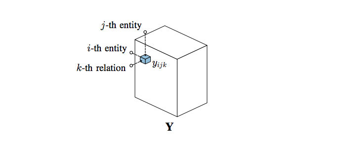
Let us say that $\textit{E} = \{e_1, e_2, ..., e_n\}$ represents the set of all entities in the graph, and $\textit{R} = \{r_1, r_2, ..., r_n\}$ is the set of all relations in the graph. Any triple, $x_{ijk} = (e_i, r_j, e_k)$ can be modelled as a binary random variable $y_{ijk} \in \{1, 0\}$. All possible triples can be grouped in a 3D array $Y \in \{0, 1\}^{N_e \times N_r \times N_e}$ [1]
The matrix $Y$ can be quite huge for most knowledge graphs. However only a few of the possible relations in the graph turn out to be true. For example, the Freebase graph contains information about 400,000 movies, and 250,000 actors, but each actor has only starred in a few movies. Another important thing to consider is that knowledge graphs often have many missing or incorrect facts. One of the main tasks in knowledge graph curation, is predicting the correctness of the link between two entities [1]
Let us say that we can represent the actor Leonardo DiCaprio, as a feature vector $ e = \lbrack 0.8, 0.2 \rbrack $. The first component in this vector corresponds to the latent feature good Actor, while the second component is the feature prestigious Award. Using this method we could represent the Oscars, with the vector $ e = \lbrack 0.1, 0.8 \rbrack $
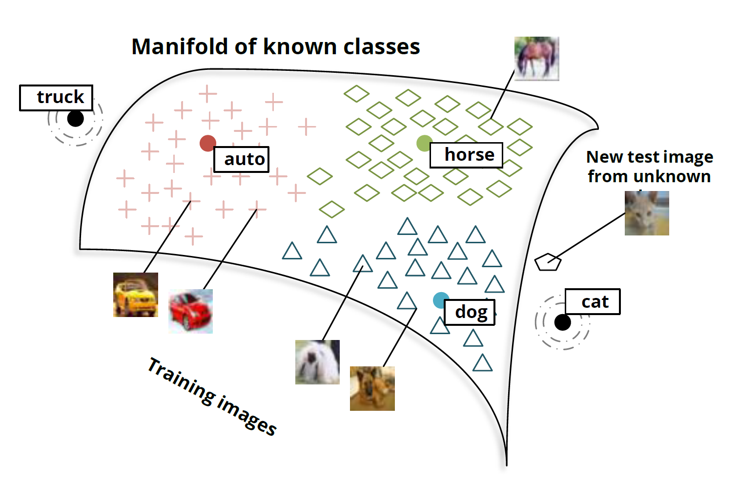
Typically, the objective of embedding methods is to organize symbolic objects (e.g., words, entities, concepts) in a way such that their similarity in the embedding space reflects their semantic or functional similarity [2]
These models try to learn features for these entities directly from the graph triples. In reality, the individual components of these learned features are not easy to intepret. The key take away from these models, is that the relationships between entities can be derived from the interaction of their latent features. They try to predict the existence of a triple $x_{ijk}$ using a scoring function, $ f(x_{ijk}, \Theta)$, which expresses the confidence that the triple exists, given the parameters $\Theta$ [1]
In this post we will examine how a simple embedding model, Fasttext, learns to represent entities in an example graph.
Dataset
We will be using the Families dataset as our knowledge graph. Our dataset consists of a total of 24 people belonging to 2 families, with 12 distinct relationships between individual members. This dataset was used by Hinton et al(1986) in their paper on the distributed learning of concepts.
# Start by importing our dataset
import pandas as pd

families = pd.read_csv('./data/families.csv', sep='\t', header=None)
families.columns = ['head', 'relation', 'tail']
families.shape
The first thing we need to do is extract the number of unique entities, in our dataset, and create a unique numerical index for each them. This index will be used later to look up the vector representation of the entity in our embedding layer. Keras provides a convenient Tokenizer API, that takes in a list strings, and creates unique integer index for each them
import numpy as np

# extract the total number of unique entities in our graph.
entities = np.unique(families[['head', 'tail']].values)
len(entities)
import json

from keras.preprocessing.text import Tokenizer

t = Tokenizer(len(entities), filters='', split=" ")
t.fit_on_texts(list(entities))

entities_index = t.word_index
As you can see below, every token in the graph dataset has been assigned a unique integer value. This value corresponds to the row representing the entity in the embedding matrix
entities_index
Next, we'll create one hot encoded labels for each relationship in our dataset.
df = pd.get_dummies(families, columns=['relation'])
df.head()
Since our dataset is quite small, we can increase the number of examples by randomly sampling 30% of the dataset and appending it our existing data
for i in range(20):
    sample = df.sample(frac=0.3).reset_index(drop=True)
    df = df.append(sample, ignore_index=True)

df.shape
Once we have enough data, we can divide it into training, validation, and test sets. For this post, I've decided to go with a 8:1:1 split, after shuffling the entire dataset.
from sklearn.model_selection import train_test_split

# shuffles the data
df = df.sample(frac=1)

tmp, test_data = train_test_split(df, test_size=0.1)
training_data, validation_data = train_test_split(tmp, test_size=0.1)
Model
We will be using Fasttext to learn our embeddings. Fasttext is a linear classification model, originally developed as a baseline for sentiment analysis. It is a simple model, with only a single hidden layer, but manages to deliver comparable performance to more complex models, and takes significantly less time to train [3]
It works by averaging the vector representations of a set of discrete tokens into a Bag of Words representation, and feeds this representation into a linear classifer that computes the probability distribution over a set of classes
Fasttext frames the knowledge based completion task as a classification problem. In our example, it will try to classify whether a given entity pair has a valid relationship. It does this by minimizing the following loss function.
Where $x_n$ is the input token, $y_n$ is our label, $V$ is the embedding matrix that represents the latent features of our entities, $W$ is the weight matrix of the classifier, that captures latent features of our relations, and $f$ is a sigmoid activation function, that acts as the scoring function.
from keras.models import Model

from keras.layers import Input
from keras.layers import Embedding
from keras.layers import Dense
from keras.layers import Activation
from keras.layers import GlobalAveragePooling1D

from keras.initializers import RandomUniform

from keras import optimizers

main_input = Input(shape=(2,), dtype='int32', name='main_input')

embedding = Embedding(name="embedding",
                      input_dim=len(entities_index.keys()),
                      input_length=2,
                      output_dim=200,
                      embeddings_initializer=RandomUniform(
                              minval=-0.05, maxval=0.05, seed=None))
x = embedding(main_input)
x = GlobalAveragePooling1D()(x)
x = Dense(12)(x)
output =  Activation('sigmoid')(x)

model = Model(inputs=main_input, outputs=output)
model.summary()

optimizer = optimizers.Adam(lr=1.0e-5, decay=0.0)
model.compile(loss="binary_crossentropy",
              optimizer=optimizer,
              metrics=['accuracy'])
We will be learning embedding vectors with 100 dimensions. The first layer after the input is just a look up table that converts our token indices $x_n$ into vector representations. The second layer averages these representations into a single vector, and then feeds it into a fully connected layer, with a sigmoid activation function for each relation.
This effectively turns our multiclass classification problem into a binary classification problem. Each output neuron in the dense layer is evaluating whether a particular relationship is valid or not.
Our model will take in a matrix of entity indices. So we will preprocess our input, by turning all the entities in the dataframe into index tokens.
X_train = training_data[['head', 'tail']].applymap(
    lambda x: entities_index.get(str(x).lower())).astype('int')
y_train = training_data.filter(regex=("relation"))

X_valid = validation_data[['head', 'tail']].applymap(
    lambda x: entities_index.get(str(x).lower())).astype('int')
y_valid = validation_data.filter(regex=("relation"))
X_train.head()
model.fit(X_train.values,
          y_train.values,
          verbose=1,
          epochs=20,
          batch_size=128,
          shuffle=True,
          validation_data=(X_valid.values, y_valid.values))
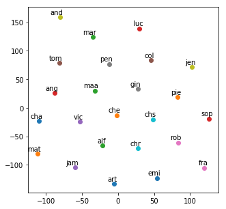
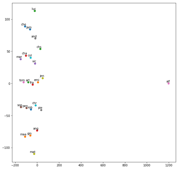
After training the model for 20 epochs, we achieve 78% accuracy on the validation set. Not bad for a baseline estimate. We can use TSNE to visualize the distribution of our embeddings in 2 dimensional space.
from sklearn.manifold import TSNE
import matplotlib.pyplot as plt

%matplotlib inline

embeddings = model.layers[1].get_weights()[0]

labels = []
tokens = []

for word in entities_index.keys():
    labels.append(word)
    token = embeddings[entities_index.get(word) - 1, :]
    tokens.append(token)

tsne_model = TSNE(perplexity=40, n_components=2, init='pca', n_iter=2500, random_state=23)
new_values = tsne_model.fit_transform(tokens)

x = []
y = []
for value in new_values:
    x.append(value[0])
    y.append(value[1])

plt.figure(figsize=(8, 8))
for i in range(len(x)):
    plt.scatter(x[i],y[i])
    plt.annotate(labels[i],
                xy=(x[i], y[i]),
                xytext=(5, 2),
                textcoords='offset points',
                ha='right',
                va='bottom')
plt.show()
# The two families are:
f1 = ['chr',
      'pen',
      'and',
      'che',
      'mat',
      'art',
      'vic',
      'jam',
      'jen',
      'chs',
      'col',
      'cha'
]
f2 = ['rob',
      'maa',
      'pie',
      'fra',
      'gin',
      'emi',
      'luc',
      'mar',
      'ang',
      'tom',
      'alf',
      'sop'
]
The TSNE plot after 20 epochs of training shows that the model is trying to separate the two families, with most of family 1 in the top half of the graph, and most of family 2 in the bottom half of the graph. This grouping has been learned directly from the data. The model has received no input on which person belongs to which family.
Before training
After 20 epochs of training
Conclusion
We implemented a baseline embedding model that was able to capture information about the individual families directly from our data. One thing to note is that this model does not effectively capture asymmetry in the relationships. The triple (Charles, father, Arthur), and (Arthur, father, Charles) would both be valid according to this model. We can circumvent this by creating a seperate embedding layer for each entity depending on whether it appears as a subject or an object.
That being said, Fasttext still provides a reasonable baseline to estimate latent features in our data. Separating the embeddings into subject and object embeddings could potentially lead to better separation of the two families, but we can explore that in another post.
References
[1] Nickel, Maximilian, et al. "A review of relational machine learning for knowledge graphs." Proceedings of the IEEE 104.1 (2016): 11-33.
[2] Nickel, Maximillian, and Douwe Kiela. "Poincaré embeddings for learning hierarchical representations." Advances in Neural Information Processing Systems. 2017.
[3] Joulin, Armand, et al. "Bag of tricks for efficient text classification." arXiv preprint arXiv:1607.01759 (2016).
[4] Hinton, G. E. (1986). Learning distributed representations of concepts. In Proceedings of the eighth annual conference of the cognitive science society (Vol. 1, p. 12).